Roll Your Own, Part 1

In my article Friends in Low Places (which can presumably be found on this blog by scrolling back far enough; here is the ProSoundWeb link), and in the identically-named chapter of my book, I showed the three basic techniques by which a cardioid-type subwoofer response can be achieved using two elements. Regular readers are also familiar with the effect of increasing line length - namely, increased directivity in that plane.

I challenge readers and practitioners not to think about this work as selecting from a mental list of “vanilla” subwoofer configurations, but rather, assembling these conceptual Legos in various permutations to create bespoke subwoofer arrangements to address particular coverage requirements.

In The Crossroads Array, I showed an example of how to utilize one particular variable - in a two-box gradient stack, are we to reverse the top or bottom? - in order to direct the front radiation and/or rear cancellation in specific ways.

In this case we expand on that concept to create yet a different coverage shape for yet a different coverage requirement. Our particular application is a concert held in a ballroom-type venue that is wider than it is deep. This is always a surprisingly difficult coverage shape to create, typically approached by a broadside subwoofer line with a heavy delay arc to widen the coverage pattern.

However, in this case, logistical limitations restrict us to a Left/Right placement for the subwoofers, on either side of the 42’ wide stage. Although I do not share the strong aversion to all L/R subwoofer deployments that many of my colleagues have, it is certainly far less than ideal with the particular audience geometry we have in this case, as the power alley coupling creates a narrow lobe down the center of the venue, and less energy on the sides, which is the opposite of what we want.

The first step is to create a bit of low-end rejection on stage. Since the subs will be placed on either side of the stage, a vanilla cardioid that cancels directly behind the array is not the ticket here – rather, we want to steer the cancellation off to the side and land it on the middle of the stage where the artists are.

That means the physical cabinet reversal must happen in the left-right plane, not the front-back plane. To accomplish this, I stood all four subwoofer enclosures up on their sides with the most onstage unit facing rearwards. (If you do this with 2100-LFC as I did in this case, be mindful to remove the rigging pins and “tuck” their lanyards out of the way as you stand the subwoofer up, otherwise you will crush them beneath the enclosure.) We then connecting the rigging links between the cabinets on the top side to lock the deployment together.

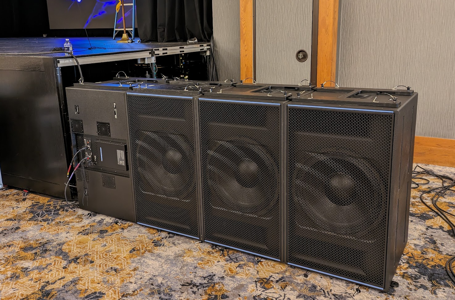
FIGURE 1 - a photograph of the stage left array as deployed

To predict this arrangement, rather than placing four individual loudspeakers in the software, you can save yourself some trouble by inserting it as a single flown array with 4 cabinets, reversing the bottom cabinet, and then spinning the entire thing on its side.
The conceptual vector analysis tells us that we should expect a cancellation steered onto the stage with this arrangement, and that is in fact exactly what we get. 

FIGURE 2 - Isometric view of stage right array with vectors

From an alignment standpoint, I started with the delay time indicated by the manufacturer’s rear-facing preset for that element, and then massaged it by hand from there. With the microphone placed on stage, I measured the three forward-facing elements, stored that trace, then measured just the rear facing element. Since the forward-facing energy is arriving from three units all further away than the rear-facing energy (and further away by different amounts), the delay needed on the rear-facing unit was slightly more than the delay value in the preset starting point.

Note: It bears mentioning that these configurations work by manipulating the relationships between the front and rear radiation of multiple cabinets, and should not be expected to work with “single box cardioid” elements which use internal rear-firing drivers to create cardioid coverage from a single cabinet - simply because the rear radiation is required for these types of arrays to work as intended, and single-box cardioid elements have significantly reduced rear radiation.

We also have an unequal fight here – we are expecting a single rear-facing element to go toe to toe against the rear radiation of the other three – it’s not a fair fight. We will get a more effective cancellation – and a bit more gas out front – by increasing the level on the rear-facing cabinet a few dB to bring it closer in line with the level contribution on stage from its front-facing peers. In this case, I observed that a 2 dB level increase was necessary to level-match the forward facers.

But we must be careful here – it is often cautioned that level offset between elements in subwoofer array can result in unpredictable behavior when the rig is pushed hard, because some elements will limit before others. If you are expecting to wring every single dB of SPL from your PA, this is a venture best avoided. However, the overall output of the subwoofers was far in excess of what I needed to bring it into the desired balance with the full-range mains, and my final tuning had them turned down by 7 dB, meaning the rear-facer was operating at a gain of -5 dB. We had headroom to spare, so I am not at all concerned about the small level offset within the array, and in fact during the show, the array never even came close to full output.

FIGURE 3 - plan view prediction of stage right array, 50 Hz, 1/3 oct, 3 dB / color

So now we see – and prediction confirms – that this half of the array is doing exactly what we were hoping for. Can’t we just fire up both sides and move on to the next task? No. Due to significant overlap between Left and Right sides, the combined result is undesirable, creating a savage power alley pile up in the middle of the space and thinning out energy on the sides. This is the opposite of what we’re shooting for.

FIGURE 4 - Plan view, both sides, 50 Hz, 1/3 oct, 3 dB/ color

To assuage this, I implemented a rather crude version of an age-old technique first introduced to me some years ago by FOH engineer Jim Yakabuski (although I have a vague memory of Dave Rat showing me a version of the technique using 5-band analog PEQ’s in his FOH rack sometime back around 2011), using complementary EQ filters to alternatively emphasize and de-emphasize frequencies between Left and Right sub arrays. Although there are a number of approaches to subwoofer decorrelation, I have never been a fan of the time-domain implementations as they cause significant degradation to the array’s impulse response. Jim’s approach used an alternating series of high-Q boosts and cuts on his Lake processor. I implemented a lower-Q version of the same idea on the system’s GALAXY, which offers a minimum PEQ bandwidth of 0.1 oct. This is just as well, as the extremely narrow PEQ boosts can disproportionately increase the resonance of certain frequencies, causing an unpleasant ringing if program material lands right on one. I also used a lower-gain version, limiting the boosts / cuts to +/- 6 dB.

If we want, say eight PEQ filters spaced evenly (on a logarithmic frequency axis) throughout the sub range, from 25 Hz to 90 Hz, we can calculate the frequency spacing coefficient by finding the 7th root of 3.6. (90 Hz / 25 Hz is a frequency ratio of 3.6, and we want to start at 25 Hz and land at 90 Hz divided into 8 filters, or 7 hops.) The 7th root of 3.6 is very nearly 1.2. Starting at 25 Hz and multiplying repeatedly by 1.2 gives us filter centers at 25 Hz, 30 Hz, 36 Hz, 43 Hz, 52 Hz, 63 Hz, 75 Hz, and 89 Hz, give or take some rounding here and there. We use same F and Q for both sides, but complementary gains: where one side boosts, the other side cuts.

FIGURE 5 - decorrelation filters

Giving one side the level advantage at a given frequency means the arrivals at the center of the venue are no longer “equal level” and so the combined summation is greatly reduced.

This is, like everything else, a trade off. Or, more accurately, several. How much gain to use is a tradeoff. More filter gain means more decorrelation but increased audibility of the filters. You have a similar call to make when it comes to filter spacing and Q (resonance). To quote the Arbiter, we trade one villain for another. And of course we need a bit more headroom in the subwoofers. The nice thing about this method is that you have it “on a lever” - it’s not just on or off. You can dial down the filter gains if it is deemed too audibly objectionable, and get back a little more power alley as a trade off. (The converse is also true: you can “dial up” or “dial down” the power alley to accommodate preference.) It’s also possible to disable the filters entirely if it’s not worth the tradeoff in that particular space. But as we see below, it reduces the combing to a single lobe just off center, and the depth of that null has been reduced by 9 dB.

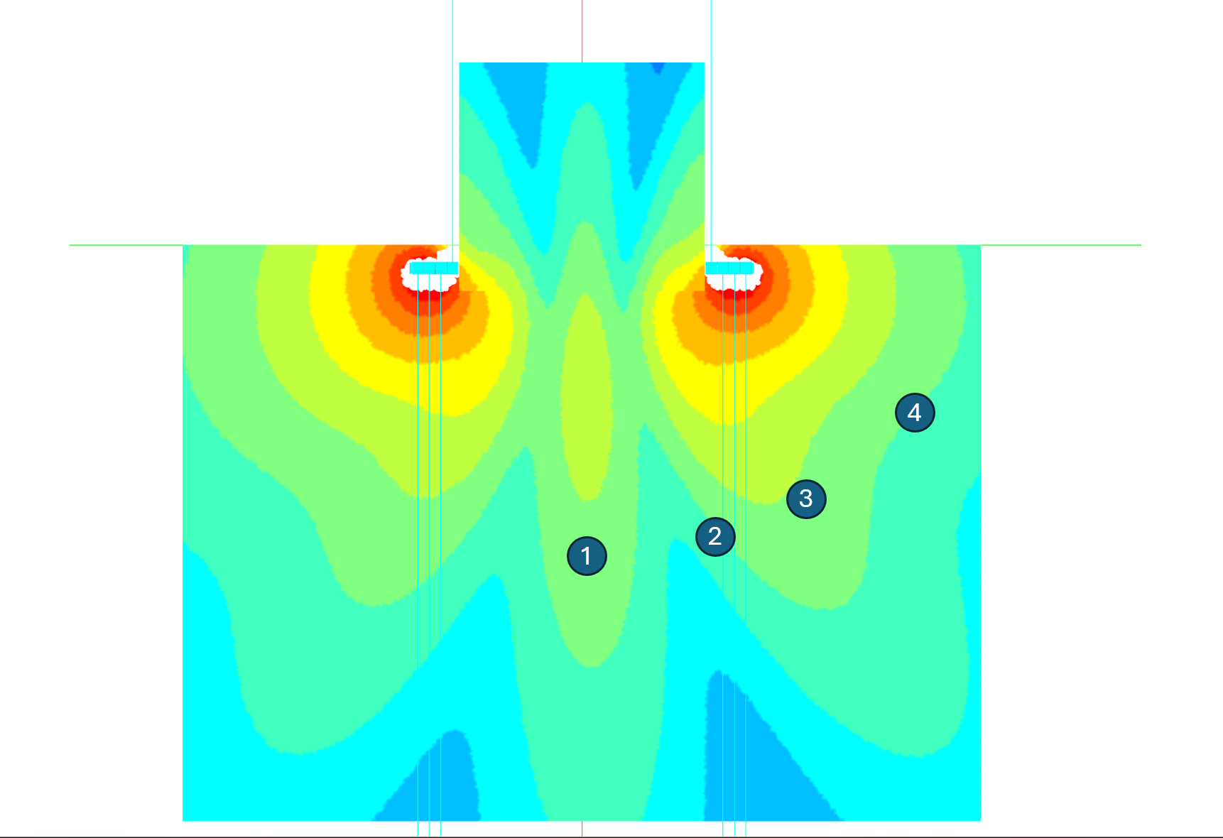
FIGURE 6 - the result, with approximate mic positions for data in FIGURE 7

Most importantly, there’s no level buildup on center at mix position compared to the listeners seated further off to the sides - we have +/- 3 or 4 dB along any given arcuate distance from the stage - and thus our lowest octaves now make a shape that is a much better match for the HF coverage shape made by our mains and outfills. If additional width was needed, the outermost element in each array could be delayed a touch, but after listening to the deployment, I decided I liked it as-is.

This is also a prime example of “it looks worse than it sounds.” Remember a prediction shows a single frequency range, and that’s not how we hear. Removing the level build up on center and drastic drop offs on both sides means that listening while walking the above-described arc results in a lot more perceptually even coverage, as the large overall level variations from center to outside edge are significantly reduced. After all, any time we put subwoofers in a room with walls, we introduce narrow-band rippling much like these filters (intentionally) introduce, and for the most part they tend not to be overly objectionable, but of course, that’s up to you.

FIGURE 7 - Magnitude response measurements of the array with both sides on, taken along the approximate positions shown in FIGURE 6. No normalization, 1/6 oct smoothing. The filter ripple starts to become more prominent as the mic moves away from center. The overall level is extremely consistent between all positions.

Like other techniques, it’s simply one more tool in the tool kit, and it’s easy to bail out of - if you implement it, and don’t like the way it sounds, you can turn it off.

Also, one additional technical note - not all DSP are created equal when dealing with very narrow filters in the LF range, so it is advisable to measure your processor directly and make sure the filtering down there is doing what it says before implementing the technique in the field.

The intended takeaway here: combining a variety of established techniques and principles to create an array that meets specific design goals.