Steer Me Right, Part 2: Principles In Practice

In the previous installment, we learned the basic concepts of how to apply delay to elements in an array to steer the coverage, and studied the effects of that steering on the impulse response, as smearing caused by spreading the arrival times. (If you’re jumping straight in here at Part 2, it might be beneficial to review Part 1 first, as Part 2 builds off those concepts.) Let’s begin this exploration by understanding the problem we’re trying to solve.

In FIGURE 1 below, we can see an example of an asymmetrical coverage challenge, where we need more output towards the top of the array to reach the farther listeners. This is easy to accomplish in the high frequency range by using the appropriate splay angles (see Beyond Coverage Angle for more) but as the figure confirms, the low-mid coverage will always emanate from the geometric center of the array. In many common geometries, this is not a pressing issue, but in a situation such as this, where we need rather asymmetrical coverage, we could achieve higher uniformity if we had a way to steer the low-mid lobe upward so it was a better match for the HF. In other audience architectures, it’s possible that the low-mid lobe may end up pointed in the right direction, but too severely narrowed to match the HF shape well.

In other geometries, a combination of both problems may manifest. In all cases, the issue is the same in general terms: the low-mid coverage shape of the array is not a good match for the HF coverage shape. While the short wavelengths at high frequencies respond well to splay angles and the directivity of the horns and waveguides (magnitude steering), the array elements are highly overlapped at LF and so “steer by committee” (phase steering). Anything we do to try to rectify this issue in the low mid must therefore rely on the interaction between the elements to create the desired beam shape.

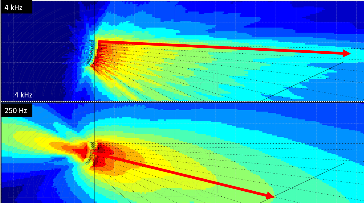
FIGURE 1 - The coverage at 4 kHz is an excellent fit for the audience geometry, but the 250 Hz coverage shape is not keeping up.

Of course, we could try to do this mechanically by tipping the entire array upwards, however that would result in all the HF going in the wrong direction, so that’s not a good tradeoff.

We can apply what we learned in Part 1 by applying delay incrementally up the array, with more on the top boxes, to try to steer that low-mid lobe upward. We used a handful of milliseconds to do this steering in the sub range. Two octaves (4x the frequency) above that at 250 Hz, we’ll have to use a quarter of the amount of the delay time to get a comparable effect. So let’s try a 0.25 ms taper per box, which means box 12 at the bottom of the array starts at 0 ms, and box 1 at the top ends up with 2.75 ms.

FIGURE 2 - A 0.25 ms delay taper at 250 Hz

This actually works brilliantly! The coverage shape at 250 Hz is now an excellent match for the 4 kHz shape. Only one small problem - it’s completely destroyed the behavior of our system higher up in the spectrum. That 0.25 ms delay offset is only an eighth of a cycle (45°) offset at 250 Hz, which is why it works so well for steering, but it’s causing mayhem in the higher frequencies - for example, we now have adjacent array cabinets firing a full cycle apart at 4 kHz. That delay time creates a different phase offset at different frequencies, completely disrupting the summation behavior and steering energy off in weird directions. It also - and this is kind of important - sounds terrible, because we’ve effectively built comb filtering into our sound system.

FIGURE 3 - Delay taper causes destructive effects in the frequency response

So what we need is a way to apply phase offset per element in the low-mid region to accomplish the steering, but without disrupting the response at higher frequencies. We can’t use delay for that - we have to use filtering, and specifically, filtering that can give us frequency-dependent delay. We need to, in essence, electronically make the top boxes of the array further from the listeners at lower frequencies, which should give us the same coverage steering effect as tipping the array upwards, but without disrupting the HF behavior, which is already mechanically optimal.

About This Investigation

The remainder of this article is an examination of the steering tech used by three leading loudspeaker manufacturers: Meyer Sound, d&b Audiotechnik, and L-Acoustics. I have attempted to include ‘explainer’ resources from all three manufacturers we’ll be examining here - I think it’s important to understand how the manufacturer has explained their toolset before doing our own evaluations of it.

An important note: everything discussed here is based on information made publicly available by the manufacturers and what is indicated in the measurement data presented below, and similar data can be produced by anyone with access to the equipment. The explanations and conclusions presented here are simply my educated guesses based on measurements and established engineering principles, and may be incomplete or incorrect - I have not requested review or comments on this article from any of the manufacturers. I feel that it is part of my professional responsibility as a systems engineer to understand the tools we use in our work, and this investigation is my own exploration into that understanding. Readers are advised to draw their own conclusions based on the available information, and to consult the manufacturers in question for guidance on implementing these tools. Opinions presented are my own.

In addition, a practical caution is in order: directly measuring audio amplifiers involves high voltages that can be potentially harmful to both yourself and your audio interface - if you choose to undertake a similar study, proceed with care!

Low Mid Beam Control

We start by looking at Meyer Sound’s low-mid beam-steering solution, termed Low Mid Beam Control (LMBC). Here is a brief “explainer” video that recaps the issues we’ve examined so far, as well as introduces Meyer Sound’s solution in the form of LMBC.

LMBC uses staggered all-pass filters per element to create phase offsets in the low-mid region without disrupting the higher frequencies. Important note: the all-pass filter itself is not what causes the steering - any processing that is applied equally across the entire array doesn’t change directivity. The mechanism here is that the all pass filter is tuned to a slightly different frequency per element, and that small phase offset between elements in the low mid region is what steers the coverage. As we move forward, keep in mind that in all cases, the absolute phase response of the array, or the loudspeakers within it, is not of interest here - what makes the steering work is the difference in phase response from element to element, so that’s what we should focus on. By measuring each channel of the GALAXY loudspeaker processor directly, we can study the filtering.

FIGURE 5 - Low Mid Beam Control filtering

True to its name, the All Pass Filter has no effect on the magnitude trace. By rolling the phase trace 180° we can gain a more intuitive look at the staggered filtering. (Phase data is cyclical but a phase plot is a 2D graph so graphing it adds an edge somewhere, just like the difference between a globe and a map - there are no dragons off the edge of the map - it is seamless data - so too with the phase trace).

Here, the filtering creates about 17° of phase offset between elements at 250 Hz (equivalent to a delay taper of about 0.2ms) but the traces converge above and below that, causing minimal disruption at HF. Note that filter spacing will vary based on the LMBC parameters, but the mechanism is clear. What we have is frequency-dependent delay between elements in the low mid range, which is responsible for the steering. Setting the mode to “Beam Spread” would taper from the middle of the array outwards in both directions, instead of a taper from top to bottom as we see here. Keep this in mind - we’ll see it pop up soon.

The biggest benefit of LMBC in my opinion is that the controls and the filter parameters are viewable for evaluation and adjustment by the systems engineer. That is, you can see exactly what it’s doing, because the APF are displayed in the Compass control software, and a user can adjust the LMBC parameters while watching the filters move around, and can modify the behavior as they see fit. Having the filter parameters displayed also means it’s straightforward to apply matching filtering to supporting systems (say, front fills) and opens the door for “out of the box” use cases.

A few examples: since the LMBC dialog displays the “average” APF parameters, I sometimes tweak the LMBC parameters for side hangs until the filtering lands on the same center frequencies, thus ensuring that the main and side hangs have a closely matched phase response and the transition region is smoother. This is, like all things, a trade off, but I appreciate the flexibility to make this call on a case by case basis as I feel is best for the situation at hand.

I’ve also been able to successfully use LMBC to “steer up” on a main array that was driven as a hybrid: 2-box zones at the top of the array and 1-box zones towards the bottom. Since LMBC requires the user to specify 1 or 2 box zones per array, it can’t natively support this configuration, but since it shows you where the filters should go, I was able to generate what the filter parameters would have been for 2-box zones, and simply add them manually as appropriate to generate the same steering effect on my hybrid zoned array.

It might be a benefit to some that LMBC uses all pass filters, which invoke no additional delay into the transmission chain, unlike the FIR filters we’re about to see in other implementations. However, I find this to be less of a concern in the context of large-format PA systems, where the propagation through the air is the majority shareholder in transmission time, unlike monitoring situations where low latency is critical.

The biggest drawback of LMBC in my opinion is that it’s inherently limited: “steer up” is limited to array splays of 45 degrees or less, although there are ways to cheat that when desired, and although the two options are “Steer Up” or “Beam Spread,” sometimes neither is a complete solution. It all depends on the geometry you’re trying to cover, and in general, LMBC ends up being a more useful tool in sheds, amphitheaters and outdoor stages, where trim heights are relatively low and curvature is generally less, and I find it less useful in arenas where trim is higher and curvature is generally more extreme (it is not uncommon for a main array in an arena environment to have 75° of splay or more).

Take a closer look at the prediction above, and notice that the rear lobe is steered up as well. Beamsteering is like opening or closing an umbrella, and it will steer your side and rear lobes along with the main coverage lobe. We will revisit this point later.

Some people may also find the phase wrap introduced by the all-pass filter to be a drawback. If having a phase-linear loudspeaker system is important to you, then you probably don’t want to sully that by adding a wrap. Remember that the phase response is related to the time domain response (impulse response) of the system, and that larger portions of the spectrum having a flat phase response mean that more of the frequency range is arriving all at once, and all of the products that use LMBC are phase-linear throughout most of their bandwidth as far as I know.

As we are about to learn, the FIR implementation used by other manufacturers avoids adding a phase wrap at the cost of some delay. However, the associated loudspeakers are not phase linear to begin with. In my opinion this is “six of one, half dozen of the other.” In my personal opinion, the IR smearing as a result of the different per-box responses that we get when applying any sort of beamsteering is a far more audible issue than whether the loudspeaker in question has a phase wrap, but more on that later.

ArrayProcessing

Next on the list is the ArrayProcessing feature from d&b Audiotechnik. Here is the ‘explainer’ video - hopefully you will notice some common themes compared to the previous video - we are, after all, seeking to address the same issue in both cases.

According to the accompanying technical document, “ArrayProcessing creates individual sets of FIR and IIR filters for every single cabinet of the array, each of which requires a dedicated amplifier channel.” If you are not familiar with the concept behind FIR filters, you may wish to check out my article Conceptual Explanation of FIR Filters and then come back. The gist of it is that FIR filtering allows us to manipulate magnitude and phase independently, at the cost of delay. According to d&b’s materials, ArrayProcessing adds 5.9 ms of delay to the signal chain - hardly a concern for most situations in my opinion.

To evaluate the mechanism, I created a similar venue and array architecture as the above example, and engaged a few ArrayProcessing slots, taking transfer function measurements of the amplifiers directly. I examined the effects on two different models of loudspeaker in two different array / venue configurations, and our focus here is on the general effects of enabling ArrayProcessing rather than evaluating its performance in each particular case. Evaluating the results is the purview of the system designer - our interest here is how it works. The following data shows the results of “Intrinsic” mode, which is the mildest form of ArrayProcessing in that it matches the natural front to back level drop of the array, rather than attempting to offset it electronically.

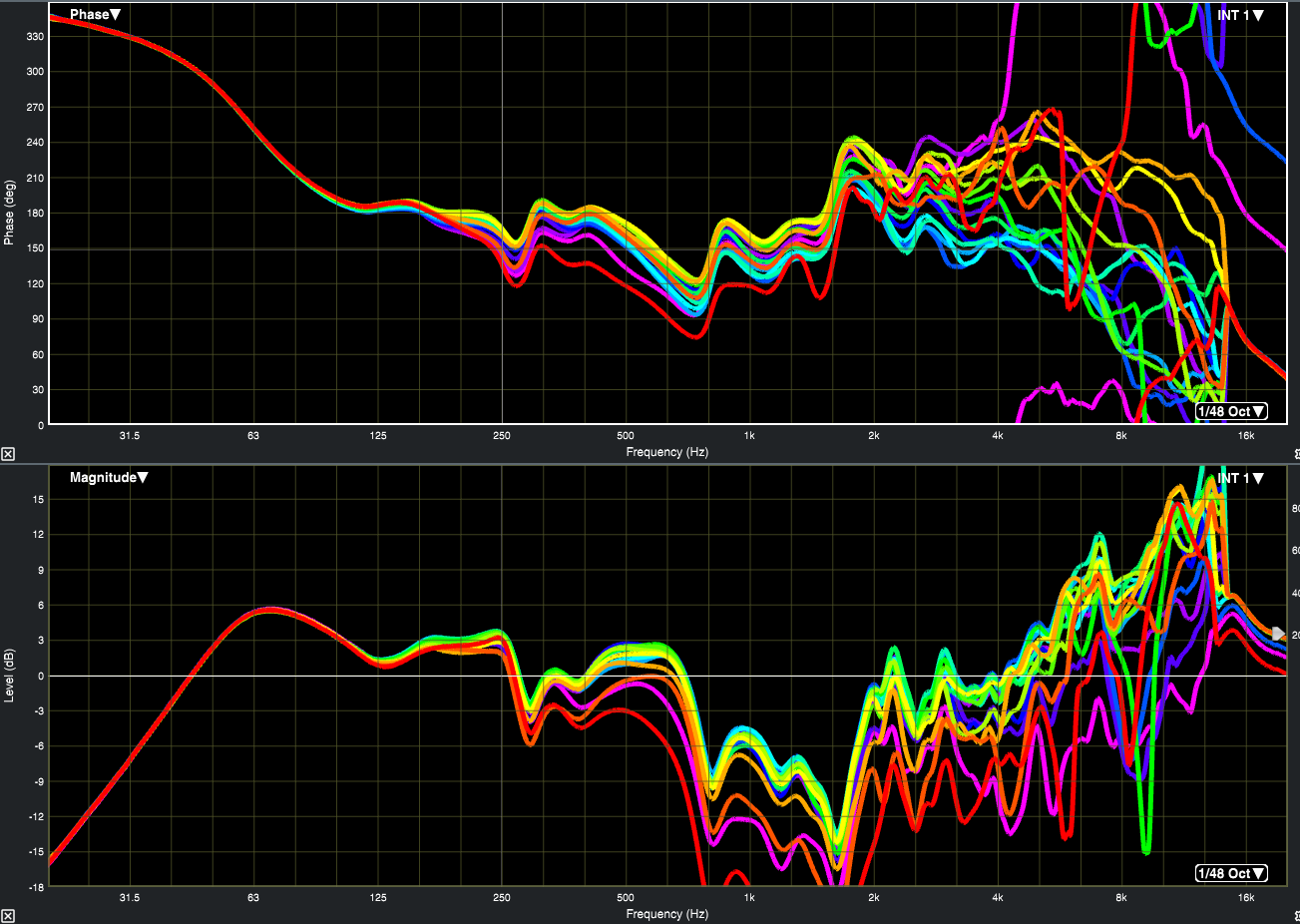
FIGURE 7 - ArrayProcessing filters + native loudspeaker preset (V8) for a 12-box array on Intrinsic mode

There’s a lot to look at here, but remember that since we’re measuring through the amplifier / DSP directly, we are seeing not only the AP filters but also the “stock” manufacturer loudspeaker preset. We can eliminate the particular loudspeaker preset from the equation by exporting the “vanilla” (AP disabled) preset as a weighting curve, and then applying the inverse of that weighting curve to the magnitude traces of all these measurements. This will subtract out the response of the loudspeaker preset, and allow us to isolate and view just the changes that AP filtering makes to the response of each element.

FIGURE 8 - ArrayProcessing filters isolated

This is a little easier to parse - we can see that the processing is not limited to the low-mid band and instead extends up to approximately 13 kHz. As noted in the above-linked white paper, the processing includes air absorption effects and HF uniformity in its calculations which explains the HF filtering we’re seeing. As an overall trend the processing has boosted HF overall, which would cause a perceptually brighter sound compared to it being disabled. Although the magnitude shading is interesting, our primary interest here is the phase offset between elements in the low-mid band.

Focusing our attention to the phase trace in the region between 250 Hz and 1 kHz, we see a familiar mechanism - a slight difference in phase between elements serving to widen and shape the directivity as the algorithm sees fit. This is accomplished without adding a phase wrap, and somewhat independently of the magnitude response - this is what has been bought by the addition of the 5.9 ms of delay for the FIR filters to do their thing. Interestingly the amount of phase offset between elements seems to remain more or less constant for a range of about 2 octaves, which sidesteps an inherent compromise of steering via all pass filter. There is also some magnitude offset in this range, but the phase offset is the majority shareholder of the steering force in the low-mid region of a line array. That being said, I did find the element-to-element response changes to be rather more severe than I would have expected given the filtering “constraints” described in the technical documentation.

It also occurs to me that this would be an excellent opportunity to phase-linearize the loudspeaker cabinet above 250 Hz or so - since FIR filtering is already in use, the necessary phase correction could be rolled into the same filtering without incurring any further delay, so I have to imagine there is some technical limitation in the implementation preventing this.

According to the technical documentation, the ArrayProcessing algorithm is “independent of array length, curvature, and system type. Any ArrayProcessing line array design will provide the same sonic characteristics.” Although I do not have extensive firsthand experience evaluating this claim for numerous combinations of loudspeaker products, it is a welcome one because matching various system zones (mains, side hangs, front fills, etc) that are often comprised of different line lengths and different loudspeaker products typically requires some attention from the systems engineer.

ArrayProcessing can only be engaged when driving elements in single-box zones, which reduces the “pixelation” problem described at the conclusion of this article.

The ArrayProcessing dialog within ArrayCalc software includes a helpful Result tab showing the difference in magnitude response at impact points from front to back with and without the processing enabled.

FIGURE 9 - The RESULT display from the project file corresponding with the measurement data shown above.

It seems that the algorithm only looks at the on-axis impact points (aka “landing strip”) and doesn’t seem to consider audience geometry impacts spanning the entire horizontal coverage of the horn, so some of the more severe deep cuts may be less than ideal in practice, and perhaps stricter “constraints” on the algorithm to further limit how far an element’s response can deviate at any given frequency from that of its upstairs and downstairs neighbors would potentially increase coverage uniformity off axis and also further preserve headroom. Applying more drastic processing to try to reduce the front-to-back level variance of the designs I tested in turn produced more drastic filter responses, as one might expect.

Engaging ArrayProcessing also forces the user to implement air compensation, which is something I prefer to adjust manually on portions of the system rather than implementing a global change to the entire PA, because once the show starts I do not want any changes happening to the portion of the PA that the FOH engineer is mixing off of unless they directly request such a change - I just want to adjust the far-reaching elements of the system to keep in lockstep with what it sounds like at mix position.

It would be nice to have the option to restrict the filtering to the region below 1 kHz, to restrict the processing solely to low-mid beam steering, without having it affect the overall tonality of the PA or the high frequency shading. LMCB is inherently limited to the applicable frequency range, and the ArrayIntelligence Optimization algorithm from Adamson offers the user an option to restrict processing bandwidth, whereas ArrayProcessing locks out per-amplifier EQ controls. (There is a somewhat time-consuming workaround for this.) As a general policy, I try to avoid using any functions that lock out the systems engineer from adjusting processing settings as they see fit. I consider this a limitation considering that the implementation doesn’t allow the user to see or adjust the actual filtering being implemented into the system, just the predicted results.

Full Range AutoFilter

On to examining the Full Range Autofilter feature in L-Acoustics Soundvision. Some clarification is in order here: the AutoFilter in its early incarnation is simply an algorithm that attempts to increase HF uniformity by adjusting HF FIR filters per amplifier zone. The more recent iteration extends the filter effects to low frequencies. As of the time of writing, I was not able to find any written technical documentation from the manufacturer about the Full Range Autofilter, but I did find this webinar in which it is explained. (The video is embed-blocked so click through to watch it on YouTube.)

Seeing as engaging the full-range autofilter increases the delay through the system, and that it observably does not add a phase wrap to the response, we can surmise that it uses FIR filtering to stagger phase response per amplifier zone in the low-mid region. Since we are dealing with a three-way cabinet, it’s a little harder to see in the data, because the steering region around 250 Hz spans the LF and MF “ways” of the amplifier processing, so we’ll see a pair of traces this time. 6 traces for the 12-box array driven in 6 zones of 2 elements each. Remember - the exact model of loudspeaker here is not our interest - we are looking for how the response changes from zone to zone, which is the steering tool at work.

FIGURE 10 - Full Range autofilter + loudspeaker presets for LF and MF bands

Again we see the familiar spreading of phase response per zone. Interestingly this filtering seems to be focused on a lower range than the previous tools we’ve examined - phase traces diverge between 80 Hz and about 500 Hz, and ride together below and above. The zone to zone spread is about 20 - 25° at 250 Hz, which is higher than we have observed up until this point, but this is likely owing to the fact that the processing is applied in 2-element zones in this case, and I suspect the “steps” would be even larger when applied to a circuit of three elements per amplifier. As we will discuss shortly, there are some drawbacks to using such physically large zones, as the acoustic “pixels” start to become the same scale as the wavelength they’re attempting to steer.

One benefit to this particular implementation is that the HF FIR filtering (not measured for this exploration) is user-accessible and can be adjusted manually or disabled completely as desired without affecting the low frequency steering. This is a more ideal implementation in my opinion - limit the electronic steering to the frequency range over which it is required, and leave the HF shading and air compensation open to adjustment by the systems engineer if desired. This makes it much easier and more convenient to adjust to changing environmental conditions in certain portions of the system coverage, or respond to HF inconsistency - quickly and easily without disruption of coverage elsewhere.

However, I feel that the user-facing implementation is lacking, in that the current control is either on or off, with no way as far as I can tell to adjust the behavior of the steering beyond setting the coverage start and stop. This is surprising given the transparency of the HF portion of the autofilter, especially since the AutoFilter technology is described in the manufacturer’s training slides as as “No 'black box' - all settings accessible / adjustable”. And, as with above, no way to see the actual filtering being applied. My firsthand field experience with this tool is rather limited so I don’t have much to say about it in terms of user experience.

Beamsteering - General Benefits and Drawbacks

In general, the benefit of these tools is obvious: it helps more of the energy go where we want it to go, and is a helpful tool to increase coverage uniformity in situations where mechanical solutions fall short. “Point the loud side toward the audience” is the principal tenet of sound system design, and these tools can help us do just that.

Inherent drawbacks are twofold - by “inherent” I mean that they are due to the mathematical realities of electronic beam steering, not a platform-specific drawback that could be resolved with a new software feature, etc. These are general considerations, not manufacturer-specific drawbacks.

Impulse Response Smearing

First: we pay a penalty in the time domain by implementing electronic steering, as we’re manipulating the arrival time of energy on a per-element basis, and Part 1 of this series showed us how that smears the impulse response of the system. How severe or objectional this IR smearing is depends on a few factors - first, the preferences of the mix engineer. Some are bothered by it, some are not, as is true about most things in audio.

In a technical sense, the variables are overall array curvature (how much work we’re asking the steering to do) and the “acoustic resolution” of the steering. IR consequences typically become more pronounced as overall array curvature increases, and as the zones get bigger. I find it less objectionable with less array curvature, single-box zones, and smaller-format loudspeakers (because the acoustic centers are closer together with respect to the wavelength being steered), whereas I find it more objectionable when the array has more curvature, is comprised of physically larger loudspeakers (15” rather than 12” cabinet height), and processing resolution is lower (2 box zones rather than 1).

This makes sense acoustically as well: single-box zones of a 12” array cabinet give us acoustic “pixels” that are less than 1/3 of a wavelength wide at 250 Hz. Two-box zones of a 15” cabinet are 3/4 of a wavelength wide. Think about how well a subwoofer array sums when the elements are spaced by a third of a wavelength, compared to when they are spaced by 3/4 of a wavelength, and you will see the inherent tradeoff here in side lobes and combing.

In addition to being audible, this IR smearing is measurable, but it is difficult since we are primarily talking about steering / smearing the low-mid frequencies, and the impulse response measurement mathematically gives far more emphasis to the high frequency range (3/4 of the FFT bins reflect the content of the top 2 octaves). This could be studied in the field with a high resolution IR measurement (large FFT, period-matched stimulus and lots of averaging) and then band-limiting the resulting IR to the low-mid region with a user-defined filter. A project for another day. In the meantime, I would like to see the inclusion of Impulse Response data in more manufacturers’ prediction platforms; it is currently only in one out of the three studied here.

Related note: regardless of how it is accomplished, if you are widening the dispersion of your system in the low-mid range, you are also decreasing the Direct:Reverberant ratio, which may have a perceptible impact on the perceived impact or “tightness” of the system. In the strictest sense, this is not a penalty invoked by beamsteering itself, but rather the natural results of deploying a wider directivity (lower Q) system in a reverberant environment. Regardless of the cause, it could contribute to a mix engineer’s perception of the results.

Side Lobe Behavior

Recall in Figure 2 how the rear lobe moved as well as the main lobe. This is an often-overlooked side effect of electronic steering, and care should be taken to educate yourself about what is coming off the sides and back of the array, and how it will respond to the steering you’re about to implement, before dumping unanticipated energy into reflective side walls or onto the stage. Although this behavior is an inherent reality of electronic beamsteering, not all loudspeakers behave equally off-axis, and not all prediction software platforms allow you to easily evaluate these effects, so in my estimation it would be fair to say that some products and ecosystems may pose a greater concern here than others.

Conclusion

In closing, this investigation helped me gain a deeper insight into what these toolsets do, and how they do it, which allows me to make a more informed decision about when or when not to deploy them in the field. As with any investigation, many questions remain, and readers are urged to explore further from this jumping-off point.