Fuzz At The Bottom

Let’s examine the purpose and process of array shading and see if we can understand an often misunderstood issue.

Figure 1 shows the response at four mic positions on axis to the coverage of a large-format line array in an arena, before (top) and after (bottom) high frequency shading.

FIGURE 1 - A large format array measured ONAX from four locations, before (top) and after (bottom) high frequency shading.

Above 4 kHz, air absorption increasingly takes effect (Fig 1 top). Although regular readers will recognize my familiar color coding - green, orange, pink, yellow from farthest to nearest - we can also deduce the distance that each measurement was taken from the system by looking at the amount of air absorption occurring in the high frequency range. Green is the farthest throw (168 ms), and is suffering the most loss. Yellow is much closer at the bottom of the array (72 ms) and shows much more HF as a result.

Whether applied by hand via HF EQ filters, or by some automated air loss compensation system, the goal is the same, to end up with more uniform HF from front to back (Fig 1 bottom). Note that the goal is not always to completely eliminate HF loss, and sometimes we simply want to reduce it, but that’s a conversation for another day.

Although the above is a very successful example of shading, sometimes it may seem like it just won’t quite get there. The extra brightness at the bottom of the array can’t seem to be eliminated by EQ’ing the HF out of those boxes. The first few dB of shading are successful, and then that HF bump seems to stop responding to additional EQ cuts. What’s going on?

Answering this question requires a brief brush-up on one of the key concepts in line array theory: time offset. In the lower frequencies, elements are effectively omnidirectional - that is - the energy from multiple sources is highly overlapped. (FIG 2, left half) Put another way, regardless of what seat you choose to sit in, you’re listening to the entire array at LF. Out in front of the array, the arrivals from all the elements are sufficiently close in time with each other that the LF energy from each box combines constructively, creating a summation. (FIG 2, right half).

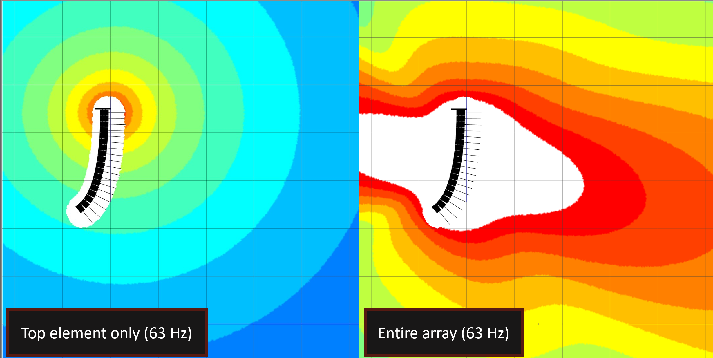
FIGURE 2 - A single element (left) and the entire 18-element array (right) at 63 Hz

Above and below the array, the arrival times from each element are sufficiently staggered to scramble the energy arrivals such that we don’t enjoy a nice, coherent summation as we do in front of the array. The longer the line gets, the more time offset we have in the arrivals and the more the pattern narrows.

If we are positioned directly above an array that’s 10 feet long, for example, the energy from the bottom box arrives almost 10ms behind the energy from the top box. Longer lines mean more time offset above and below, and the LF directivity increases. Line length is therefore the major player in determining the directivity of the array at low frequencies where elements overlap their output. Want a narrower LF dispersion? Increase the line length.

This is, in a nutshell, why trying to EQ low frequencies from a single element in an array isn’t fruitful, and can in fact cause unexpected results - at low frequencies, listeners are hearing the output from all the elements, and the whole array is riding together. We treat the entire array as one source in these frequencies.

At high frequencies, we have a completely different mechanism at work. HF directivity is created by horns and waveguides, which simply focus the HF energy in the direction we want it to go by way of pointing the loudspeaker in that direction. This works because the high frequencies have wavelengths that are short enough (measured in inches) to be effectively steered by a reasonably-sized waveguide (measured in inches). FIGURE 3 below shows the directivity of a single element at 4 kHz - the loudspeaker is designed to have a narrow vertical dispersion. Compare this to the behavior of the same element at 63 Hz (FIGURE 2) and you’ll see a stark contrast.

FIGURE 3 - The 4 kHz directivity of the top element (left) and the top half of the array (right).

The tight vertical pattern of the waveguide creates a lot of isolation as we move off-axis from the loudspeaker, unlike what’s happening at LF. To combine this with the previous concept, we could say that when listening to a line array, at LF you are listening to all the elements, and at HF you are listening to only the elements pointed at you. The waveguide is pretty narrow vertically, and once you move outside of its pattern, you’re not hearing its HF output.

Since we have different elements covering different listeners at different distances, we can very effectively adjust the HF output of each element to tailor the response as needed depending how far that particular element is from the listeners it’s covering. We can boost HF towards the top of the array, on the elements that will throw through the most amount of air and suffer the most HF absorption before reaching their listeners. (Of course we try to accomplish as much of this as possible via mechanical means - properly adjusted splay angles, with more overlap and therefore more summation at the top of the array. But processing will carry us over the finish line.)

The excess of HF that often occurs towards the bottom of a large array’s coverage (scroll up and review Figure 1 again) isn’t just due to less HF absorption. There’s another mechanic at play here, and it’s not quite as well understood. Let’s see if we can sort it out.

Look again at FIGURE 3 above, particularly at what’s going on towards the bottom of the array. It’s easy to see that listeners down there on the floor are well outside of the HF coverage of the boxes at the top of the array. But that doesn’t mean there’s no energy getting down there. Horns and waveguides aren’t brickwall filters, spatially speaking. They tend to do a pretty good job focusing HF energy in the right direction, but there’s always a little bit of bleed off the edges. Some products fare better than others in this regard, but to some degree we’re simply up against physics here.

So we do have some energy from the top boxes bleeding down onto the listeners at the bottom of the array, and depending on the situation, it can be more than you might think. FIGURE 4 below shows the output of the top half of the array at 16 kHz, using a higher resolution (1/12th octave) prediction to more clearly reveal the issue.

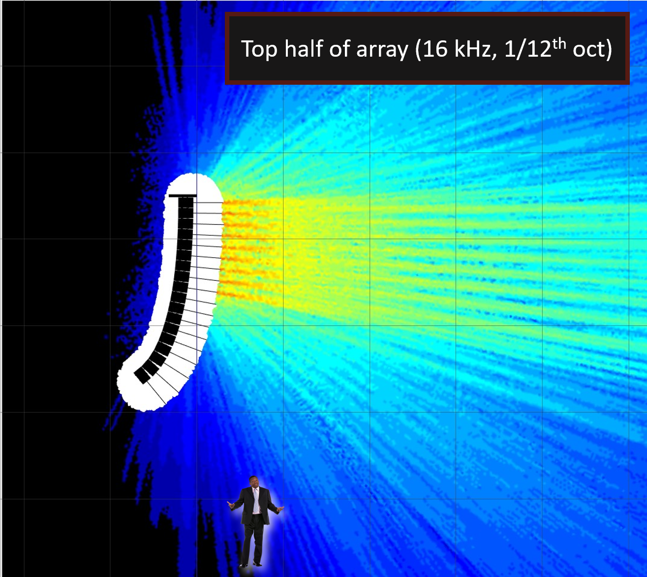
FIGURE 4 - Top half of array, 16 kHz, 1/12 oct

Our stock photo friend down towards the front of the audience area is definitely getting some of the “spray” - and so will our measurement mic.

Side note: This is an area where not all prediction software is created equal. The effect is not accurately characterized at lower frequency resolutions such as the 1/3 or 1 octave data used by many common prediction platforms, or if the platform isn’t using Complex summation math to calculate the results. In other words, don’t assume your deployment doesn’t have this issue simply because you don’t see it happening in your prediction. All prediction data in this post comes from Meyer Sound’s MAPP 3D, which uses high resolution (1/24th octave) data, complex summation, and can produce an impulse response.

What does this “spray” look like in a measurement? We’ve already seen its effects in the frequency domain - extra high frequency in the magnitude response. Let’s take a look at the time domain. FIGURE 5 below compares the impulse response of a measurement taken closer to the center of the array (top half of FIG 5) to the impulse response down at the bottom of the array (bottom half of FIG 5).

FIGURE 5 - Energy arrival (impulse response) at Onax Box 6 compared with Onax Box 16

Sharp-eyed readers will recognize these graphics from the section of my book that bears the same name as this article. What’s all that fuzz in the lower trace? That’s the HF “spray” coming from higher up in the array. It’s later in time because it’s coming from higher up, further away, and therefore arrives after the arrivals from the bottom boxes. If you’re trying to solve excess brightness down at the bottom of your array by shading the bottom boxes, you will only be successful to a point. The HF energy arriving later in time won’t respond to your bottom zone shading, because it’s not coming from those boxes. So your shading will reduce that initial sharp peak in the impulse response, but not the fuzz afterwards.

This type of thing can be somewhat difficult to study in a controlled way when working in a real-world production environment but prediction can bring some clarity here.

FIGURE 6 below shows two (virtual) measurements from the 18-box array taken from position “D,” indicated by the gold star. The red impulse response shows the IR of the entire array, while the blue impulse response is just the bottom two boxes, muting boxes 1- 16. All the red “fuzz” is the late-arriving energy attributable to the rest of the array.

FIGURE 6 - Two IR predictions from position D showing the entire array (red) and just the bottom two boxes (blue)

Let’s get a little more granular by keeping the bottom two boxes (17 and 18) turned on, and add in boxes higher up in the array, two at a time, so we can identify their contributions to the impulse response. FIGURE 7 below shows the same baseline data for the entire array in red, and the effect of unmuting boxes higher up in the array two at at time in blue.

FIGURE 7 - Unmuting boxes in pairs to identify their contribution to the IR “fuzz” measured at the bottom of the array

Now we have an answer to the question of why some of the excess HF at the bottom of an array doesn’t always respond to shading down the bottom boxes - because that energy is coming from elsewhere.

When you turn down the HF on the bottom boxes, you make things better to a point, but now you’ve reduced the direct sound by a few dB, which means more of the HF you’re hearing is coming from higher up so you’ve decreased your direct:reverberant ratio in an unhelpful way. This can lead to a weird listener experience down front in which it sounds like the bottom box is completely off. The ear has no strong direct first arrival to localize to.

Some people think they can get around this by leaving the bottom boxes as they are, and simply turning up the HF on the top boxes to match. You will begin to chase your tail with this approach, as turning up HF in the upper zones also turns up their contribution to the fuzz down low.

My approach - that seems to have served me well thus far - is to shade down the bottom zone to get as close to the desired target as possible, but once the trace stops responding, bring back one or two dB. This helps preserve the direct arrival, and gives the ear something to localize to, which seems to be the best compromise in terms of a listening experience in most cases. The amount of “fuzz” in the impulse response measurement from the bottom zone will give you an idea of how successful you can expect to be.

FIGURE 8 below shows an example of getting the bottom zone “as close as I could” - and moving on to more pressing matters. Note the Live IR fuzz for the bottom position at the top of the image. This image also appears in my book as Figure 47.

FIGURE 8 - Front to back measurements before (top) and after (bottom) high frequency shading on a large-format array. The excess high frequency energy at the bottom (blue trace) is reduced but not eliminated. Notice the ‘fuzz’ in the LiveIR from that location.