Shade and a Haircut

Today’s job is at a local 200-cap performance venue. Our task is to remove the existing PA (4 cabinets of a last-generation small-format array per side) and put up a newer PA owned by the same vendor (8 cabinets of RCF HDL-6A per side). It’s a newer, more powerful, and lighter loudspeaker and a longer line, so it’s sure to be an improvement in many ways. The venue is a simple rectangular listening area, about 70 feet from the PA lifts to the rear wall. The existing subwoofers and front fills will remain in place, so we’ll focus here on just the main arrays.

We can get a top trim of 15 feet, and we have eight cabinets. We can easily set splay angles to achieve equally-spaced impact points from back to front. One of the issues with the previous deployment is lack of overshoot - mix position at the rear of the room is not fully inside the HF coverage of the mains, so a balanced mix there translates too brightly for the audience. Here, we’ve got a bit of overshoot so that mix position is well inside the HF coverage of the mains.

*Side view of the mains, showing equally spaced centerline impacts and some overshoot at mix position in the rear of the venue.*
*Splays are 2°-2°-2°-3°-4°-7°-10°*

We are a bit limited on DSP here, and have 3 zones available for each array, so I made the decision to zone as Top 3 (A), Middle 3 (B), Bottom 2 (C). In general it’s better to have more granularity towards the bottom of the array where there’s less overlap between elements. 2-box zones would be more ideal here but 3-3-2 is probably the best compromise available given the 3 outputs.

If you’ve read my book, you know where the mic positions are going: A, B and C.

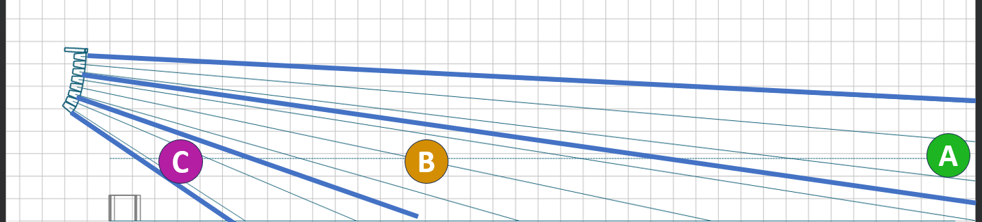
*Mic positions: ear height at the center of each array zone. Mic positions and DSP zones are joined at the hip.*

We’re working with a single mic today so let’s start by measuring the system’s performance at each location: A (66ms), B (30ms) and C (12ms). Note that I typically refer to distances in milliseconds as a shorthand.

What we have here is a textbook example of array behavior before shading - we get louder and brighter as we get closer (progression from green to pink). Normalizing the traces in the low-mid range allows us to see the HF work that we have to do if our goal is tonal consistency - our bottom zone is about 4 dB bright above 2 kHz.

*Same measurements as previous figure, normalized around 500 Hz.*

We can shave down our HF variance with some gentle HF shelving in the processing.

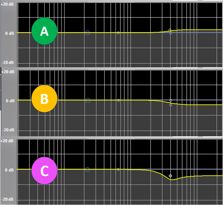
*High frequency shading for the three array zones.*

It’s, as the kids say, “super effective.” It’s easy to get caught in the details here, but such is the nature of being in a reflective space with a reflective floor. Focus on the broad strokes and we see that the HF variance is now reduced to be more akin to the LF variance. That is, it’s still louder in the front and quieter in the back but all three traces are now making a similar contour - that is - similar tonality.

Now that we have our consistency, we will add the subs back in and do some overall EQ to hit the desired tonality for system, which in this case is less LF tilt up that starts lower in frequency. We’ll do this with a combination of a low shelf cut and a PEQ cut around 200 Hz. Just a quick trim (see, now the post title makes sense.)

Notice the filters in the LF half of the spectrum are common to the entire array, while the HF filters diverge from zone to zone.

And a look at the final traces (note the different horizontal scale, now showing down to 20 Hz) with our tonality target in view (top) and the same data normalized (bottom).

Fuzz At The Bottom

Crossroads Array